Big Wheel Bot – Gardening Robot

I have been working on a project for the last few months that I am referring to as the ‘Big wheel bot’. This robot is based around some 250mm diameter wheels that I purchased and this project has evolved as its gone along. Initially I was planning to build a balancing robot but this changed into a differential drive robot with a rear castor as I had a purpose in mind for this robot. That purpose was to help in the garden. I wanted to go a step further than a lawn mower robot and I wanted something that could navigate autonomously and check on the various plants in the garden. I am working towards that goal.

I have written a post on letsmakerobots so I won’t repeat it all here but here is the link. https://www.robotshop.com/community/robots/show/big-wheel-bot

I have also made a new series of videos showing the process of designing, building and programming the robot. I am still working on this project and I have got as far as producing the first occupancy grid map with the robot.

All the code for this project can be found here: https://github.com/BigFace83/Big-Wheel-Bot

More Sensors! Sonar and MPU6050 module

I have added some sensing to the RC robot in the form of some sonar sensors and an MPU6050 IMU module. This project was always heading away from being a purely RC robot towards an automated mobile robot platform. The addition of sensing is one of the steps in this process. Adding and interfacing the sensors was quite straight forward and Part 11 of my Youtube series takes you through the process.

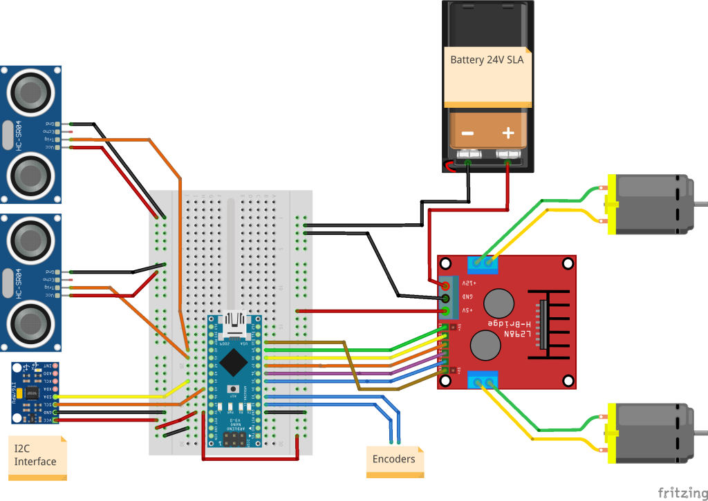
For anyone interested, here is the updated Arduino circuit I am now using.

I have also moved the HC05 bluetooth module from interfacing with the Arduino to being connected to the onboard Raspberry Pi. Partly to see if it would work but also because I want to be able to control more functions from the transmitter and it seemed to make sense to have the Pi get the data from the transmitter and send it on the to Arduino. Time will tell if this is a good solution.

The next steps will be to improve the serial communications between the Arduino and Raspberry Pi as I’m not happy with how that is working at the moment. Then I want to log sensor data to a file, along with images captured from the webcam, as the robot is being driven around. I will then use this data to work on some mapping/SLAM solutions I would like to try out.

Capturing video using a Raspberry Pi, OpenCV and Python

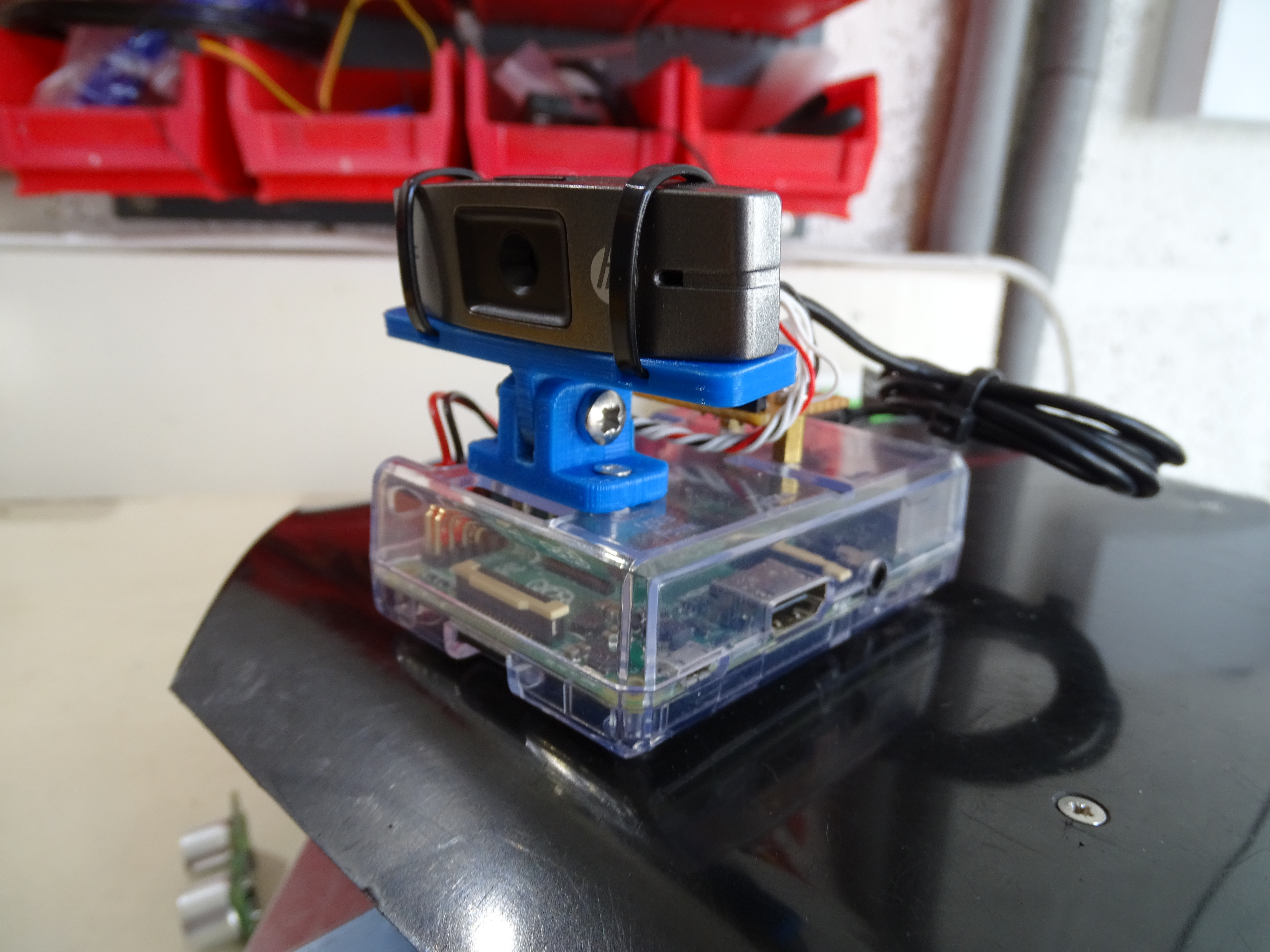
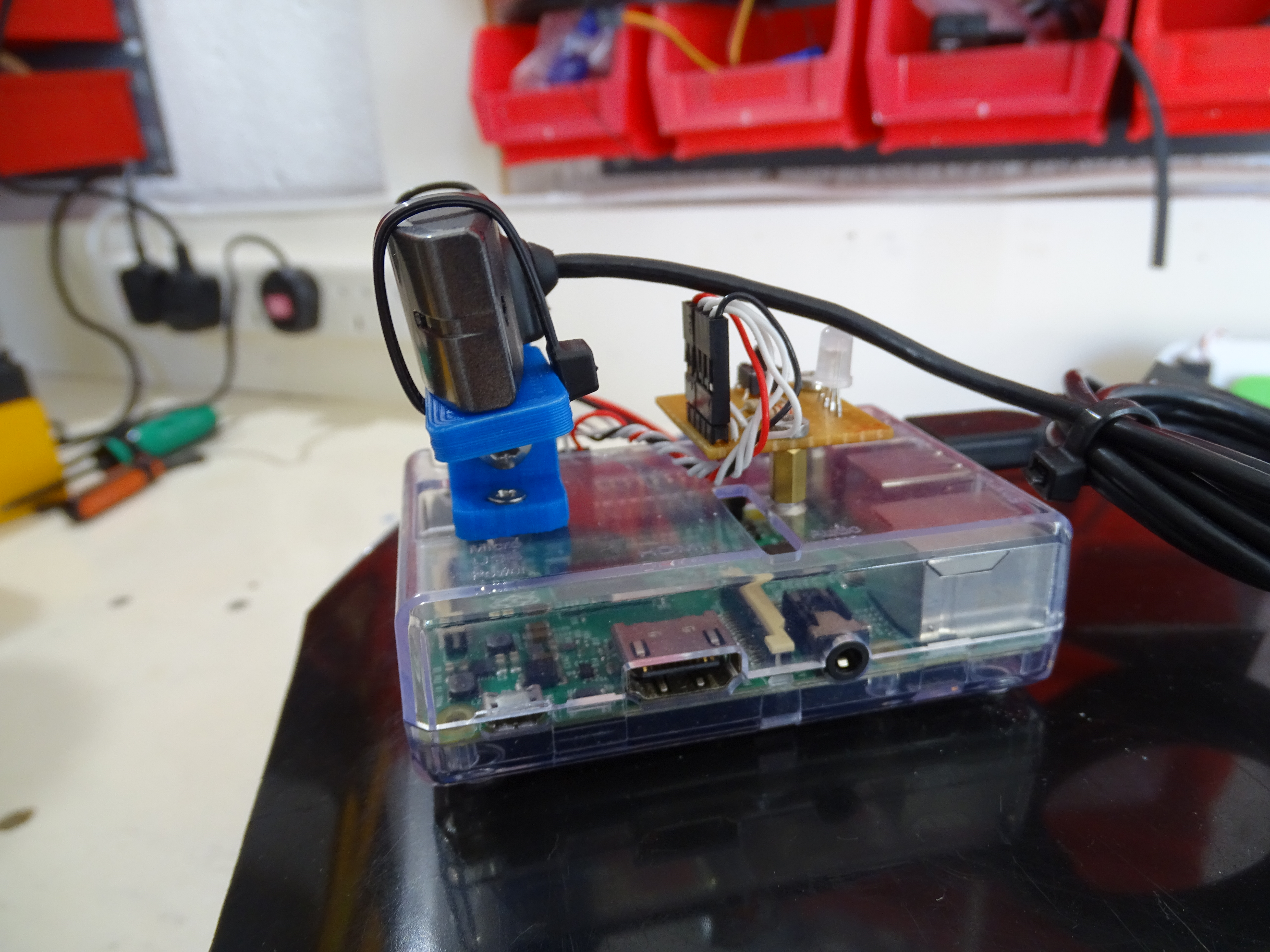
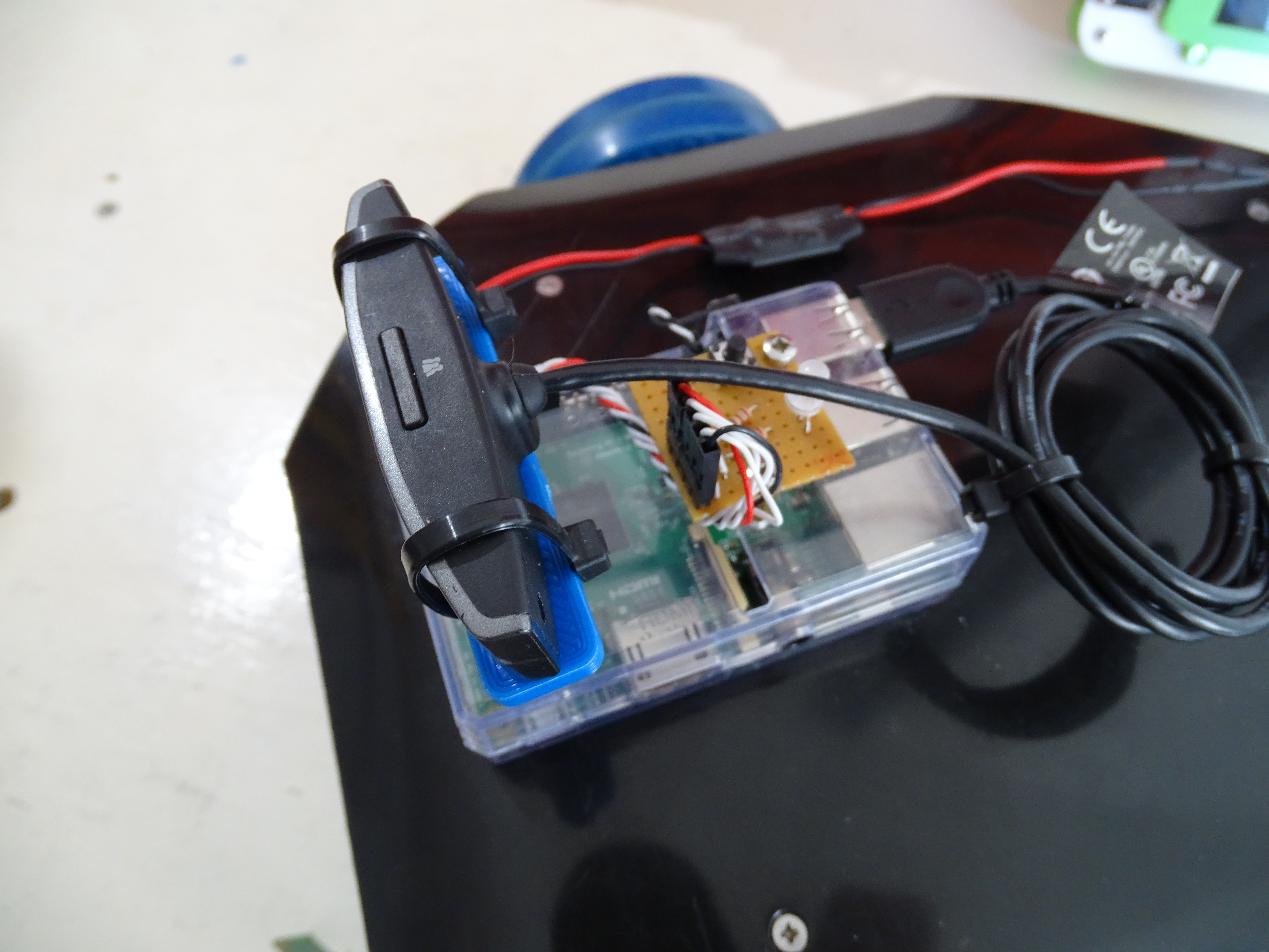
I decided it was time to add some sensing to the RC robot. The first of which was to add some vision in the form of a webcam connected to a Raspberry Pi. I had a Raspberry Pi 2 at hand so that is what I am currently using, along with a standard webcam. The aim to start with was to enable to capture of video as the robot drives around under remote control. Ultimately I plan to use the camera, along with other sensors to automate the robot. But I wanted to start simple and build from there. To keep it simple I decided to make a small circuit with  a button to start/stop recording and an RGB LED to indicate whether the Pi was recording video or not. I also 3D printed a simple mount for the camera. These components were attached to the Raspberry Pi case resulting in a compact assembly that could be attached to the robot. One other component was required and that was an additional switch, mounted to the side of the case, that would allow the Raspberry Pi to be shutdown when pressed.

• 

• 

• 

Combined with a battery pack or some other form of power this would make quite a nice stand alone project, maybe as a dashcam or any other device that needs to capture video. In may case I will be using power from the 24V batteries on the RC robot, via a UBEC connected to the GPIO pins.

The next job was to write a python script that would start and stop video capture at the push of the button and store this video for later use. I used OpenCV to capture images from the webcam and store as a video. Each video would be stored with a file name created using a time stamp. I also added the LED functionality so that the LED was green when ready to begin recording and red when recording. The last part of the code was to shut down the Pi when the shut down button was pressed, after flashing the LED a few times to indicate that the button has been pressed. I set it up so that this script runs on start-up of the Pi. The full code is shown below.

import time
import os
import numpy as np
import cv2
import RPi.GPIO as GPIO

print "Starting..."

GPIO.setmode(GPIO.BCM)
GPIO.setwarnings(False)
GPIO.setup(22,GPIO.OUT) #Red LED
GPIO.setup(27,GPIO.OUT) #Green LED
GPIO.setup(17, GPIO.IN, pull_up_down=GPIO.PUD_UP) #Button Input for recording
GPIO.setup(21, GPIO.IN, pull_up_down=GPIO.PUD_UP) #Power off button

recording = False

print "Starting OpenCV"
capture = cv2.VideoCapture(0)

imagewidth = 640
imageheight = 480
capture.set(3,imagewidth) #1024 640 1280 800 384
capture.set(4,imageheight) #600 480 960 600 288

# Define the codec and create VideoWriter object
fourcc = cv2.VideoWriter_fourcc(*'XVID')

cv2.waitKey(50)

def CaptureSaveFrame(outfile):
    ret,img = capture.read()
    ret,img = capture.read() #get a few frames to make sure current frame is the most recent
    outfile.write(img)
    cv2.waitKey(1)
    return img

def LEDGreen():
    GPIO.output(22,GPIO.HIGH) 
    GPIO.output(27,GPIO.LOW)
    
def LEDRed():
    GPIO.output(22,GPIO.LOW)
    GPIO.output(27,GPIO.HIGH)

def LEDOff():
    GPIO.output(22,GPIO.HIGH)
    GPIO.output(27,GPIO.HIGH)

def CreateFile():
    timestr = time.strftime("%Y%m%d-%H%M%S")
    print timestr
    out = cv2.VideoWriter('/home/pi/Video_Recorder/'+ timestr +'.avi',fourcc, 5.0, (imagewidth,imageheight ))
    return out

def Shutdown(channel):
    print("Shutting Down")
    LEDOff()
    time.sleep(0.5)
    LEDGreen()
    time.sleep(0.5)
    LEDOff()
    time.sleep(0.5)
    LEDGreen()
    time.sleep(0.5)
    LEDOff()
    time.sleep(0.5)
    LEDRed()
    os.system("sudo shutdown -h now")

GPIO.add_event_detect(21, GPIO.FALLING, callback=Shutdown, bouncetime=2000)

LEDGreen()

while True:

    input_state = GPIO.input(17)
    if input_state == False:
        recording = not recording #Toggle bool on button press
        time.sleep(1) #Debounce
        if recording:
            LEDRed()
            out = CreateFile()
        else:
            LEDGreen()

    if recording:
        CaptureSaveFrame(out)

Part 10 of my Youtube video series shows the robot in action and capturing video as it drives around.

This set-up works great and I have already started work using the video and OpenCV to see how I can get the robot driving around autonomously using the video input. I will also be adding some additional sonar sensors to the robot for obstacle detection/avoidance as I don’t want to rely on the visual input alone to avoid crashes! I also intend to reconfigure the robot control so that the Raspberry Pi is the master of the system and the Arduino is the slave, taking commands from the Raspberry Pi. Thats it for now, thanks for taking the time to read this and I’ll be back soon with more updates to the project.

Homemade RC Controller and PID wheel control

With the RC robot test drive completed it was time to make a more permanent solution for the hand held controller. I designed and built a controller with 2 analogue control sticks and a TFT screen, powered by rechargeable NiMH batteries. Inside there is an Arduino Nano with a HC-05 module for bluetooth communications to the robot. I used some expanded PVC sheet along with 3D printed parts to make a case. Part 6 of the RC Robot video series shows the build of the controller.

I was really pleased with how the controller turned out. It works really well and fits in the hands nicely.

With the controller build completed, I turned my attention to the software for controlling the robots wheel speed. Initially I just had the wheel speeds controlling proportionally to the joystick positions. This worked ok but I wanted to implement closed loop speed control with feedback from the incremental encoders. I also wanted to be able to control the robot using only one of the analogue joysticks, which turned out to be trickier than I had first thought.
Part 7 of the video series covers the PID control and converting the control to using only one analogue joystick, along with some fun testing of the robot in the garden.

I really struggled to work out how to control the two wheel speeds and turning using just a single analogue joystick until I found a great explanation that can be found here http://home.kendra.com/mauser/Joystick.html
This page explains the theory, and the equations that pop out at the end enable the wheel speeds and directions to be calculated based on the input from the single analogue joystick.

After some more testing of the robot with the improved control software it became clear that the robot had a few design issues. The main one being that the robot was a real handful to control accurately. It is great fun to drive but I need to be aware that I am making a robot platform, not an RC car. One issue was that the robot was simply a bit too quick. This was easy enough to remedy by limiting the PWM output to the motor driver to limit the top speed. I also noticed that when you released the joystick, the robot had a tendency to continue rolling for a bit, due to its momentum. This sometimes didn’t matter too much but sometimes one wheel would continue while the other didn’t, putting the robot off course. I turned on motor braking on the motor driver when the joystick was centred and this helped a bit but didn’t cure the problem.

Therefore I had some decisions to make about the next steps of the project. I will go into more details in my next blog.

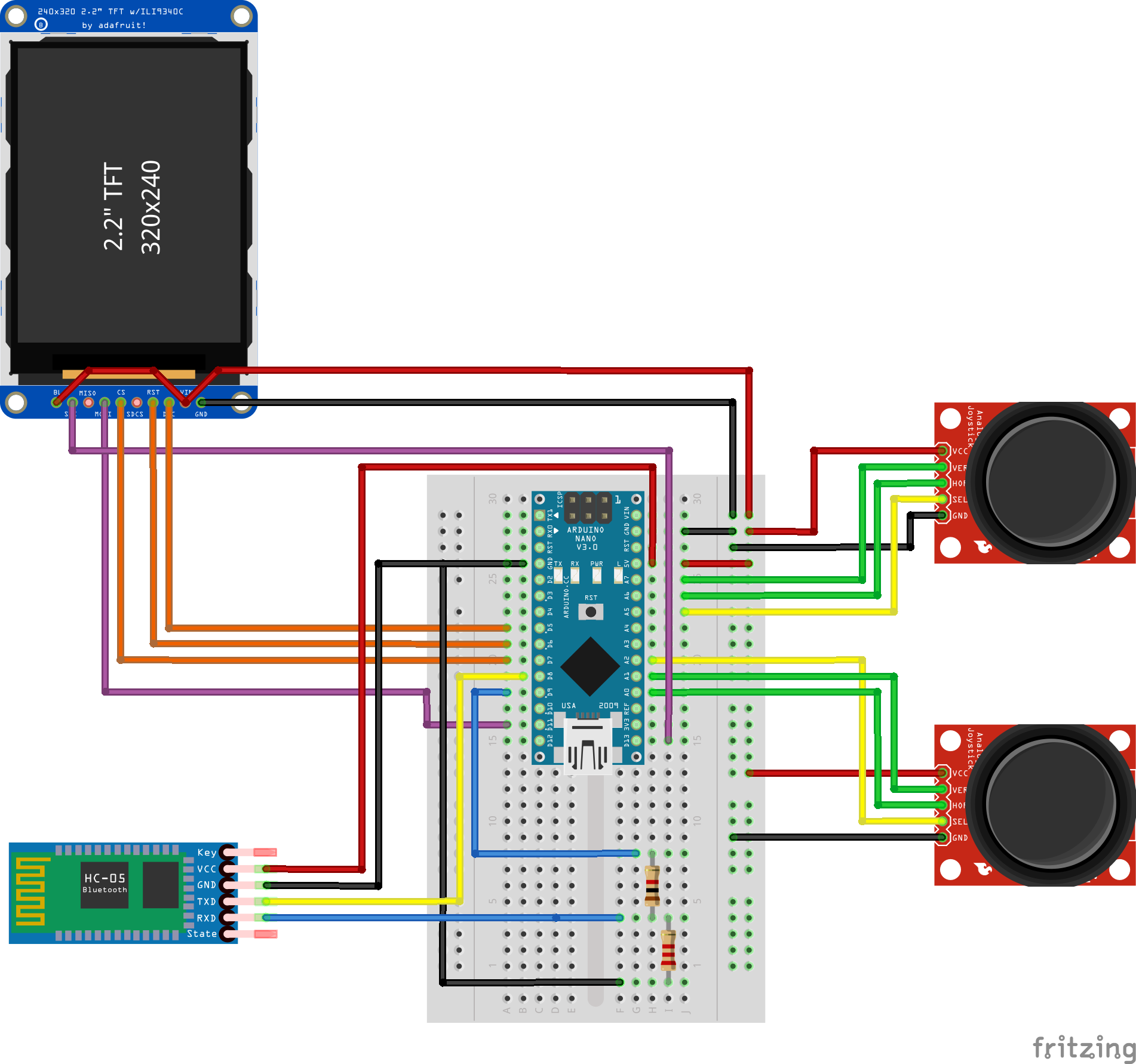
EDIT:  I have been asked to share the design and code for the controller so below is the circuit I am using.

I have also been asked to share the code. Other than writing to the TFT screen, the code is pretty straight forward. The joystick positions are read using an analogue read and then this data is formatted into a string to be sent via the serial port. I am using a software serial port to send data through the HC05 module as this keeps the main serial port free for debugging. I wanted to keep the data sent from the transmitter as simple as possible and the work of decoding and using the data is performed by whatever is receiving the data.

#include "SPI.h"
#include "Adafruit_GFX.h"
#include "Adafruit_ILI9340.h"

#include <SoftwareSerial.h>
SoftwareSerial BTSerial(8, 9); //  TX,RX

#if defined(__SAM3X8E__)
    #undef __FlashStringHelper::F(string_literal)
    #define F(string_literal) string_literal
#endif

// These are the pins used for the UNO
// for Due/Mega/Leonardo use the hardware SPI pins (which are different)
#define _sclk 13
#define _miso 12
#define _mosi 11
#define _cs 7
#define _dc 5
#define _rst 6

#define XCENTRE 506
#define YCENTRE 528

Adafruit_ILI9340 tft = Adafruit_ILI9340(_cs, _dc, _rst);

const int LeftButton = A2;     // the number of the pushbutton pin
const int RightButton = A5;     // the number of the pushbutton pin

String X = "X";
String Y = "Y";

const int LeftXin = A1;  // Analog input pin for left joystick X
const int LeftYin = A0;  // Analog input pin for left joystick Y
const int RightXin = A6;  // Analog input pin for right joystick X
const int RightYin = A7;  // Analog input pin for right joystick Y

int prevLXDisplay = 0;
int prevLYDisplay = 0;
int prevRXDisplay = 0;
int prevRYDisplay = 0;

void setup() {

  tft.begin();
  delay(300);
  tft.setRotation(3);
  tft.fillScreen(ILI9340_BLACK);
  delay(300);
  tft.setCursor(20, 60);
  tft.setTextColor(ILI9340_BLUE);  tft.setTextSize(6);
  tft.println("BIG FACE");
  tft.setCursor(20, 120);
  tft.println("ROBOTICS");
  delay(500);

  Serial.begin(9600);
  BTSerial.begin(9600); //Bluetooth software serial
  
  pinMode(LeftButton, INPUT_PULLUP);
  pinMode(RightButton, INPUT_PULLUP);
 

  while(digitalRead(RightButton) == HIGH){ //Wait right here until right joystick button is pressed
  }
  tft.fillScreen(ILI9340_BLACK);
}

void loop(void) {

  tft.fillCircle(prevLXDisplay, prevLYDisplay, 10, ILI9340_BLACK);
  tft.fillCircle(prevRXDisplay, prevRYDisplay, 10, ILI9340_BLACK);
  drawGuides();
  
  int LXValue = analogRead(LeftXin);
  int LXDisplay = map(LXValue, 1023, 0, 20, 140);
  int LYValue = analogRead(LeftYin);
  int LYDisplay = map(LYValue, 0, 1023, 60, 180);
  
  int RXValue = analogRead(RightXin);
  int RXDisplay = map(RXValue, 1023, 0, 180, 300);
  int RYValue = analogRead(RightYin);
  int RYDisplay = map(RYValue, 0, 1023, 60, 180);

  tft.fillCircle(LXDisplay, LYDisplay, 10, ILI9340_RED);
  tft.fillCircle(RXDisplay, RYDisplay, 10, ILI9340_RED);
  prevLXDisplay = LXDisplay;
  prevLYDisplay = LYDisplay;
  prevRXDisplay = RXDisplay;
  prevRYDisplay = RYDisplay;

  int XValue = (XCENTRE-RXValue)/2;
  if (XValue < -255){
    XValue = -255;}
  if (XValue > 255){
    XValue = 255;}
  
  int YValue = (YCENTRE-RYValue)/2;
  if (YValue < -255){
    YValue = -255;}
  if (YValue > 255){
    YValue = 255;}
 

  // print the results to the serial monitor:
  String XString = X + XValue;
  String YString = Y + YValue; 
  Serial.print(XString);
  Serial.println(YString);

  BTSerial.print(XString);
  BTSerial.println(YString);


  delay(100);


}

void drawGuides(){
  //tft.drawLine(x1, y1, x2, y2, color);

  int LeftCentX = 80;
  int LeftCentY = 120;
  int RightCentX = 240;
  int RightCentY = 120;
  
  tft.drawLine(LeftCentX, LeftCentY, LeftCentX-60, LeftCentY, ILI9340_WHITE);
  tft.drawLine(LeftCentX, LeftCentY, LeftCentX+60, LeftCentY, ILI9340_WHITE);
  tft.drawLine(LeftCentX, LeftCentY, LeftCentX, LeftCentY-60, ILI9340_WHITE);
  tft.drawLine(LeftCentX, LeftCentY, LeftCentX, LeftCentY+60, ILI9340_WHITE);

  tft.drawLine(RightCentX, RightCentY, RightCentX-60, RightCentY, ILI9340_WHITE);
  tft.drawLine(RightCentX, RightCentY, RightCentX+60, RightCentY, ILI9340_WHITE);
  tft.drawLine(RightCentX, RightCentY, RightCentX, RightCentY-60, ILI9340_WHITE);
  tft.drawLine(RightCentX, RightCentY, RightCentX, RightCentY+60, ILI9340_WHITE);
  
}

Population coding neural network

This was an interesting weekend project that I completed a few months ago. I challenged myself to write some slightly different code for my robot head that would lead to an interesting visual representation of the robot head position. Partly inspired by real neural networks in the brain, I used population coding of a large number of neurons to represent the head pan and tilt position. I was able to extend this further to actually control the head position. Check out the video below for a more in depth description.

 

Template matching and tracking

I have been playing around recently with template matching and locking on to a target with the Robot Head MK 2. Parts 6 and 7 of the video series about this robot are available on Youtube.

 

After a training session where the user manually identifies and names a template, the robot can now match the template in the current image from the camera. The head will then move to centre the detected template in the robots field of view. The 3D position of the object is then calculated using the robot model and the reading from the sonar sensor. I have got as far as plotting these positions in a 3D matplotlib plot.

It was at this point that I noticed some problems. Its known that sonar sensors have a wide beam angle and this is particularly apparent when the robot is looking at something far away. The issue manifests itself as objects being detected as closer than they actually are, due to the wide beam of the sonar detecting objects that are either side of the head, closer than the target object. I could combat this with a different, probably more expensive type of sensor but I am going to try a different approach.

As explained in Part 7 above, I don’t really need a 3D model to show the robots head position, as this can be represented in pan/tilt coordinates. Whilst I have learned quite a bit from playing with template matching, its not the best method for matching scenes that the robot sees. It doesn’t work at different scales and its susceptible to false detection’s. I am going to try something different and I’ll be honest, I’m not sure what just yet! I have always been interested in how mapping works in the brain, and I think what I am trying to achieve  is similar to RatSLAM. On with some more reading and research and I will be back with an update again soon.

 

WXPython GUI

Part 5 of my video series following the development of a desktop robot head was uploaded a couple of weeks ago. The video covers more progress on the robot head project including constructing a new circuit board for the Arduino Nano to replace the prototype breadboard circuit. This video shows the GUI built using WXPython that can now control the robot. OpenCV images and matplotlib plots have been embedded in the GUI and some initial image processing and robot modelling functionality is working.

 

 

I am now thinking carefully where I go next with this project. What I really wanted to try next was coming up with a way for the robot to identify objects of interest in the environment and log these, adding them to some kind of map/plot. From here the robot can then try and find these objects again using the camera to locate itself within the world. This isn’t a new idea but I am not sure how to progress yet. OpenCV has inbuilt functions that can identify good features to track and several algorithms to match these points to what a camera is seeing. However, these are quite abstract points; corners, edges etc. I would like to robot to be able to pick out objects from the environment, that a human could also identify. To do this I think there will need to be a training step, where a person looks at an image and tells the robot that an object is present. Then I can use something like template matching to identify the object in the future. In theory as this is a static robot, the angle and distance to objects shouldn’t vary too much and this technique may work. It’s something I want to try, and I will be sure to let you know the outcome.

The next question is; What next? I always reach this stage with all of my robot projects. I really enjoy designing and building robots, and it’s a rewarding experience when the robot comes to life and starts moving around. But I am the first to admit that my creations are somewhat useless. As a learning experience and a fun hobby, they are a worthwhile endeavour, but they are never created with an end goal in mind.  Maybe this is something to address in my next robot project!

 

Point clouds using the robot arm

Several months ago I posted the final video (Part 8) in the series looking at the build of a Desktop robot head and arm.  I say final video as, for the time being, I have shelved this project and have moved on to something else. I learnt a lot from this project and I will likely revisit it at some point in the future.

The video above takes you through the process of using the robot arm, along with the model described in the previous post, to build a point cloud representation of the robots surroundings. I added feedback to the final servo in the robot arm assembly, the sonar tilt servo, and I was then able to calculate the position and orientation of the sonar mounted on the end of the robot arm. Using the sonar reading, I could then apply the same technique used to calculate the robot joint positions to find the x,y and z coordinates of the object that the sonar was detecting. This position could then be stored as a point. I programmed the robot arm to move to a series of positions and record a measurement from the sonar sensor as a point which was added to a large array. This array could then be plotted as a 3D plot in the matplotlib window in the GUI.  I pushed this as far as I could and ended up with a point cloud of several thousand points. At this point my PC was struggling to display the points and allow the plot to be rotated or zoomed smoothly. The gathering of the data for the largest point cloud I created took somewhere in the region of 30-40 minutes.

The point cloud experiment was interesting as it showed that the position of objects could be estimated and stored as positions in an array. One of the reasons that I moved on from this project was that I wanted to revisit previous work of combining a distance sensor with a camera. I would like to be able to capture an image, extract one or more objects of interest from the image and measure a distance to the object. This information can them be stored in some form. Similar to the way the point cloud represents distance points, I would like to build up a cloud of objects and their positions that the robot can later use to reference what it is currently seeing.

I will be back very soon with another post as I have made good progress with the next project that I will be sharing here.

Modelling the robot arm – Denavit Hartenberg parameters

Part 7 of my Youtube series, documenting the building and software development of my desktop robot head and arm, is now available.

 

I have designed a new attachment for the end of the robot arm. For the time being I have removed the touch sensitive ‘hand’ and I have replaced it with a sonar sensor, mounted via an additional micro-servo. The idea is that the sonar can measure the environment and use this information, in conjunction with the camera mounted i the head, to build up a visual and spacial model of its environment. I’ll be honest, I’m still a bit fuzzy on how this is going to work but it should keep me busy for a while.

This episode also demonstrates the progress that I have made in modelling the robot arm. With the model in place, I have been able to generate a mimic of the robot arm, embedded in the GUI. I have used matplotlib to generate a 3D plot that I use to display the model of the robot arm.

The first step in modelling the arm, was to find its Denavit Hartenberg parameters. There are lots of great resources online that detail how this is done, so I will only cover it briefly. I assigned reference frames to each of the robot arm joints, namely the base servo, lower arm servo, elbow servo and end effector (sonar) servo. From these reference frames, and some measurements taken from the robot, I was able to find the Denavit Hartenberg parameters as shown in the table below.

 

Description	Link	a	α	d	θ
Base	0	15mm	90	102mm	θBase
Lower	1	150mm	0	0	θLower
Elbow	2	161mm	0	0	θElbow
End	3	38mm	0	0	θEnd
Sonar	4	Sonar Distance	0	0	0

 

The variables in this case, are the θ values, which are the joint angles. You will notice the addition of the Sonar ‘link’ in the table. I will explain more about this in a moment. With these values identified, it is then a case of using these in a Denavit Hartenberg matrix to find the Cartesian coordinates of each joint. Multiplying the XYZ coordinates for a joint by the successive Denavit Hartenberg  matrix, gives the coordinates of the next joint on the arm.

I was able to calculate these coordinates for the arm, initially using joint angles given by sliders in the GUI, and plot them on a 3D matplotlib plot. This was embedded in the GUI and the robot arm model moved as the sliders were altered. It was then possible to read live joint angles from the robot so that the model reflected the actual position of the robot arm at any time.

The additional sonar ‘joint’ in the table above was used to calculate where in 3D space the sonar sensor, mounted to the arm, was measuring to. I treated the sonar sensor as an additional prismatic joint on the robot and as such the variable is the distance measured by the sonar sensor whilst the angle of the joint remains constant. I was then able to plot a line that represents the sonar sensor reading on to the robot model.

I plan to do the same bit of work for the robot head and have a model of that on the screen as well. This is likely to be the content for the next video in the series. I also want to explore a way to use the sonar readings to plot the environment as the robot arm moves around. At the moment I am thinking either a point cloud type data structure or a 3D occupancy grid type approach, but this is very early days so the approach may change.

For now, please enjoy the most recent video and subscribe to my Youtube channel for notifications of future videos. Any feedback or recommendations are welcome.

Colour detection and tracking

Part 6 of my Youtube series was posted last weekend and I have been working on tracking coloured objects.

 

As mentioned in my last post, I decided to develop the tracking function using the detection of a coloured ball instead of faces. To detect a certain colour I converted an image from the webcam to HSV colours, and then applied a threshold to isolate the coloured object of interest. Using contours I was able to detect the position of the coloured ball in the image. I could then use the x and y screen coordinates of the detected ball to calculate x and y error values. Multiplying these errors by a gain value (currently 0.04) and adding each value to the current yaw and pitch servo positions, allowed the head to move to track the object. I have been experimenting with different gain values but this seems to give a reasonable result at the moment.

Using the same code, but with the threshold values changed, I was also able to get the head to track the end of the arm. Although there is always some room for improvement, this ticks another item off of the wish list.